II. Fractionation of Cell Wall Polysaccharides
III. Total Sugar and Uronic Acids
IV. Methyl Esterification of Uronic Acids
VI. Linkage (methylation) Analysis
VII. Fourier Transform Infrared (FTIR)
VIII. Protocol for the screening of the UniformMu maize population with near infrared reflectance spectroscopy
VIII. Protocol for the screening of the UniformMu maize population with near infrared reflectance spectroscopy
Wilfred Vermerris
March 2006
1. Overview of the NIR screening
We screened approximately 1,000 families (20,000 plants) of the UniformMu population per summer. The screening was performed on dried leaf segments from adult leaves, and the spectra from this population were subjected to multivariate statistical analyses to identify aberrant spectra that were consistent with the segregation of a mutation within the family. Progeny from the plants with aberrant spectra were then re-screened the next year.
2. Field design
In order to accommodate variation in the field (soil, moisture gradients), and physiological variation related to the time of day (see next paragraph), we planted W22 controls along the sides of the field and through the middle.
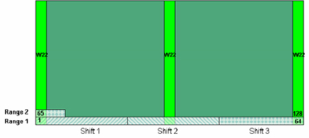
Figure 1. Field design for leaf collection and spectral acquisition. The light-green areas represent W22 controls planted along the borders and through the middle of the field. The field in this picture is 64 rows wide. The three shifts represent three teams of NIR probe operators acquiring NIR spectra (see description in section 5). Each of these shifts included the W22 controls from the range from which their leaf samples were obtained. In this example, shift 3 would include the W22 controls from both range 1 and 2.
3. Barcoding
We barcoded the plants when they were approximately 6-8 weeks old. If you do it much earlier, the tags fall on the ground when the juvenile leaves die. We printed barcodes on adhesive weatherproof white labels (Avery 5520) and stuck these on weatherproof ‘Rite in the Rain 100#’ tags. The barcode tags were stapled around the whorl, loose enough to allow growth, and low enough that the tag would stay on under windy conditions.
4. Sample collection
When the plants were approximately 1.2-1.5 m tall, we harvested a 5-8 cm section of the central part of the leaf blade of the fifth adult leaf, counting from the bottom. The distinction between juvenile and adult leaves can be made based on the epidermal wax. Juvenile leaves have a blue-ish, dull wax, whereas adult leaves have a shiny, green wax. The leaf section was cut with sharp scissors and placed in a glassine stamp envelope (#5), along with a barcode tag. This works best when a team of two people collects the samples: one person cutting, the other person filling envelopes. The envelopes were collected in big trays and dried in a 50°C oven for a week. This removes moisture from the samples, hence reducing variation in moisture content between samples, simplifying the spectra by removing a large absorbance for water, and limiting the growth of fungi.
It is important to minimize the overall time it takes to collect the samples, because the plants grow fast at this time of the year, increasing the probability of detecting developmental differences between the start and end of the leaf collection. Having a large team of people collect leaf samples is the most effective way of addressing this concern. Another source of variation is the fluctuation in metabolite levels during the day. Having W22 controls throughout the field ensures that there is always a control set relatively close by, offering a good comparison.
5. NIR spectra acquisition
The night before spectral acquisition, the envelopes were placed in the drier again, to remove any moisture that might have been absorbed. The spectral acquisition is a two-person task, whereby one person places the leaves and the corresponding barcode tag on a cafeteria tray, and the other person acquires the spectra.
We obtained the spectra using a FieldSpec Pro NIR spectrometer from Analytical Spectral Devices, Inc. in Boulder, CO (www.asdi.com). We used the hand-held contact probe to emit the light and to detect reflected light. Each leaf sample was sandwiched between a piece of quartz glass and a GoreTex ® disk. The GoreTex ® disk served as the white reference. The quartz glass kept the contact probe clean, prevented damage to the leaves, and flattened the leaf so that the quality of the spectra is more consistent. Methanol was used on a regular basis to clean the GoreTex ® disk, the glass plate and the lens of the contact probe. We used the RS3 program for the acquisition. This offered the convenience of auto-increments in the file name, so that pressing the space bar is enough to save the current spectrum and create the file for the next one. Each spectrum that was saved was based on the average of 30 individual spectra.
The spectral acquisition was handled by a team of two individuals working for a period of 3-4 hours. Approximately 20 families (400 samples) could be screened during this time.
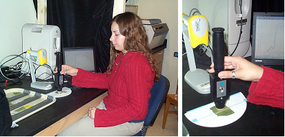
Figure 2. Acquisition of the NIR spectra from dried maize leaves using an ASD FieldSpec Pro spectrometer. The picture on the right is a close-up of the contact probe, the leaf under the gass slide, and the white reference.
The spectral data were saved digitally in a proprietary format specific for the ASD FieldSpec Pro spectrometer. The program ViewSpec allows the data to be exported into a common file format. We used the JCAMP-DX format, which generates .dx file extensions. This also allows you to save many spectra (typically generated during one session) in one single file. In order to import the data into the WinDAS analysis program, the data needed to be converted to txt format. We used a custom-designed program that converted the dx files into the correct txt format.
6.2 Data formatting
The NIR data were imported in WinDAS. Note that this package was designed for FTIR, which uses wavenumbers (cm -1) instead of wavelength (nm). As a consequence, the NIR spectrum is displayed backwards, i.e. the low wavelengths are displayed on the right of the scale. The data can be saved in tx format and imported into Excel to make graphs with the normal scale (see Figure 3). We visually evaluated the NIR spectra and eliminated any odd-looking spectra (reflectance values that are obviously too high or too low). The blue line in Figure X represents a typical NIR spectrum of a maize leaf. We then truncated the spectrum to the range between 1000 and 2400 nm (pink line) . Thus, variation in reflectance of visible light was not considered when we were looking for aberrant spectra reflective of cell wall mutations. The signal in the region between 2400 and 2500 nm is often noisy, and tended to contribute to irregularities in the data analysis. The spectra were then baseline corrected (this means that the reflectance at 1000 and 2400 nm is set to zero; green line in Figure 3), and the spectra were normalized. Normalization corrects for variation in signal strength resulting from variation in leaf size and light leaks between the glass surface and the contact probe. The truncated, baseline-corrected, area-normalized spectra were then saved in WinDAS format (.wdd file extension), and subjected to statistical analysis.
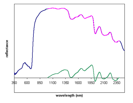
Figure 3. a typical NIR spectrum obtained from a maize leaf (blue), the truncated spectrum in the range between 1000-2400 nm (pink), and the baseline-corrected spectrum (green)
6.3 Class modeling
We started out with an unsupervised data analysis, meaning that we did not assign a genotype to the individual spectra. We started out defining a W22 wild-type ‘class’ based on spectra of W22 controls from the same area of the field that the putative mutants of interest were in. This class model, built in WinDAS, was based on a set of principal components (PCs) that were new, linear combinations of the original wavelength variables, whereby the variance-covariance structure of the data is taken into account. Each principal component that is generated captures a certain portion of the variance present in the raw data. For the class model we selected the PCs that capture approximately 90% of the variance. That typically is 2-4 PCs, depending on the exact dataset. Selecting too many PC’s can result in overfitting, which basically means that you add so much information in your model that irrelevant differences result in the rejection of samples. In essence, when you use the class model approach, you evaluate whether the spectra of the putative mutants are consistent with those of the wild-type plants. The WinDAS software will return a table in which every individual is displayed, along with a decision: accept (similar to W22) or reject (different from W22).
In order to accommodate spectral variation related to the NIR probe operator the NIR spectra of the W22 controls that were selected for the class model and the putative mutants that were to be evaluated were acquired at the same time and by the same team of people.
6.4 Genetic constraints
Rejection in the class modeling can be the result of many factors (mud, damaged leaf, fungal; growth, poor spectral acquisition, etc.). In order to consider an outlier a potential mutant, we placed a genetic constraint on the system: we want at least two outlier spectra that are different from W22 but similar to each other. In order to evaluate this, we evaluated the PCA score plot in which the spectra from the putative mutants were plotted. In the ideal case several outlier spectra consistently cluster together along all PC axes.
Figure 4 shows a set of score plots obtained from the class modeling. In panel A no outliers are identified (all samples consistent with the W22 wild-type spectrum), even though there are two individuals that are somewhat removed from the rest of the group. Panel B shows the scoreplot from a different row with a total of 12 rejected individuals, which have been marked in color (afterwards). The yellow and purple samples represent two groups that are consistent with a Mendelian segregation ratio. In this particular case we also had progeny from a sibling of the row with the putative mutants. We expect that if there is a genetic basis for the spectral variation that there would be additional putative mutants among the progeny of the siblings. Panel C shows the combined rows. Note how there is an additional set of rejected individuals (spectra not consistent with W22 controls; marked in blue) right near where the samples marked in yellow are. In contrast, there are no additional outlier spectra near the samples marked originally in purple. So in this case we would mark the individuals marked in yellow and blue. Since the spectral acquisition was carried out by a big team, the spectra can be sensitive to operator effects. We had a single individual redo all of the rows with putative mutants, along with the appropriate W22 controls. The data analysis was again performed on this new set of spectra, and only those samples that are consistently being detected as outliers were selected for the generation of homozygous mutants.
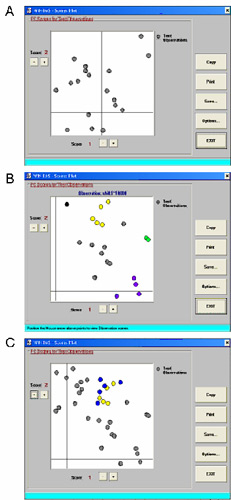
Figure 4. Class modeling of families of maize lines based on a model developed from the NIR spectra of W22 wild-type leaves. A. a family without any outlier spectra. B. A family with several individuals that are not consistent with W22 spectra (indicated in color), C. The same family as in B, plus a related family both contain individuals with spectra that are inconsistent with W22 spectra, but similar to each other (yellow and blue circles).
6.5 Data interpretation
Once we had at least five individuals representing one mutant, we compared the NIR spectra of the mutants and the W22 control to identify the chemical basis of the altered spectral properties. We went through the same spectral manipulations (truncate the spectra, baseline correct, area normalize), data compression, and discriminant analysis. The data compression was generally performed using partial least squares (PLS), which compared to principal components, resulted in better separation of the two genotypes. The loading of the most important PLS (usually PLS1) and the score plot were copied into a Powerpoint slide.
Before starting the data interpretation, it is important to consider that the NIR spectrum is a reflectance spectrum. Hence, high values (close to 1) mean high reflectance, and therefore low absorbance. Low values (close to 0) mean high absorbance, and an abundance of compounds that contain the functional groups absorbing the IR light of a specific energy (wavelength). When the PLS loading indicates that the coefficient associated with a particular variate (wavelength) has a high value (in absolute terms), that means that this wavelength is important in distinguishing mutants and wild types.
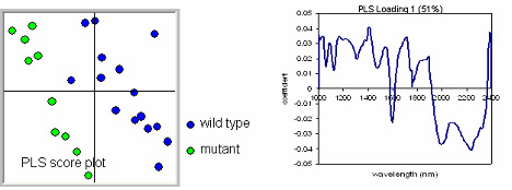
Figure 5: PLS score plot (on left) representing the individual function scores for PLS1 and PLS2 of the wild-type W22 samples (in blue), and the mutant samples (in green). The loading associated with PLS1 is shown on the right. High values (in absolute terms) in this plot represent wavelengths important for discrimination between wild type and mutant. In this example, given that the mutants cluster on the left half of the score plot, and thus have negative PLS1 values, the mutant spectra have relatively strong reflectance values at those wavelengths in the loading represented by negative values. The wild-type spectra on the other hand have relatively higher reflectance values at those wavelengths associated with positive values in the loading.
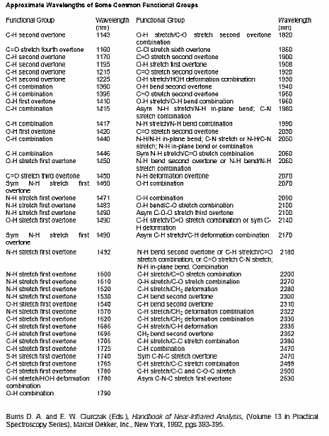
In the example shown in Figure 5, the multivariate analysis results in a negative PLS1 scores for the mutant samples. This means that the spectra of the mutants have higher reflectance values at those wavelengths that have negative coefficients in the loading and/or lower values at those wavelengths with a positive coefficient in the loading. Again, a high value means higher reflectance, and therefore lower absorbance. By identifying the functional group(s) associated with a particular absorbance, we can make some inferences on the chemical basis of the difference between wild type and mutant. In this case we observe negative peaks at 1600, 2050, and 2230 nm, and a series of positive peaks, including those at 1050, 1100, 1190, 1420, 1560, 1720, 1900 and 2390 nm. Based on Table 1 we can assign functional groups to a number of these peaks.
Table 1. Interpretation of NIR spectra
Back to top